

Showing posts with label LabView Example. Show all posts
Showing posts with label LabView Example. Show all posts
Monday, August 20, 2012
Sunday, August 19, 2012
Lab .2(d) While Loop / For Loop / Shift Register / Selectors
More than often, we would like an action to repeat until a condition is satisfied; for example, we may want to accept data from the user until the datum provided is of a particular value, at which point we stop processing any further data. This is where loop structures such as the While Loop come in handy.
 ); this means that, when we connect a Boolean control (a control that returns either True or False) to the terminal, the While Loop will stop iterating as soon as the Boolean control returns True. Another kind of conditional terminal, called Continue If True, is available by right-clicking on the conditional terminal.
There is another terminal called the iteration terminal, which is an output terminal (
 ). Every run of the While Loop is considered one iteration. During, and after, execution, this terminal returns the number of iterations completed. The iteration terminal starts off at 0; as a result, during the first iteration, the iteration terminal returns 0.
Example VI
The following exercise will demonstrate the use of a While Loop structure in a VI. This VI will keep generating a random integer between 0 and 100 in a loop until it matches a number defined by the user. An indicator will be used to count the number of iterations used to attain this match.
1. Open LabVIEW.
2. Open a new VI by clicking on Blank VI in the LabVIEW Getting Started window.
3. Save the VI as Number to Match.vi.
4. Create a random number generator, to generate integers between 0 and 100 inclusive, in a While
Loop.

• From the Functions palette, place a While Loop from the Programming → Structures subpalette.
• Using the random number generator found in the Programming → Numeric subpalette, gen-
erate a random integer between 0 and 100. Since the random number generator generates
random floating-point values between 0 and 1, use appropriate functions in the Functions palette to multiply the values by 100 and round them to an integer. You may find the Round to Nearest function useful, but you will need to look for it using the provided search functionality.
5. Create a control on the front panel that will be used to compare the results of the random number to a user-defined value, and display the number of iterations that were required to attain this match.
• From the Controls palette, place a numeric control on the front panel and label it Number to
Match.
• From the Controls palette, place a numeric indicator on the front panel and label it Iterations.
• Create an Equal? function from the Programming → Comparison subpalette and place it on the block diagram to compare the random number generated with the number present in Number to Match, as shown in Figure .

6. Create stop conditions for the While Loop.
• It is good programming practice to allow users the ability to exit a loop structure using a control on the front panel. To this effect, create a stop button control on the front panel from the Modern → Boolean subpalette.
• To also allow the While Loop to terminate when a match has been found, use the appropriate
logic functions from the Programming → Boolean subpalette to construct the necessary logic
for the stop terminal of the loop. The overall block diagram should look similar to that shown in Figure.
Notice, in the block diagram, that 1 has been added to the iteration terminal (i); this is done because iteration counts for loop structures in LabVIEW begin at 0, whereas we need to start counting iterations from 1. To create a constant (in this case, 1), right-click on the terminal and select Create → Constant.

7. Run Number to Match.vi and verify its operation. Run the VI again with the Highlight Execution button selected.
For Loop
A For Loop, like a While Loop, is a loop structure and functions similarly; the sole exception is that a For Loop performs as many iterations as determined by the count terminal (
 ).
).Example
The following exercise will demonstrate the use of a For Loop structure in a VI. This VI will generate a random floating-point number between 0 and 1 every second and repeat for a finite number of iterations specified by the user. The VI will then return the largest number generated. An indicator will be used to count the number of iterations elapsed.
1. Open LabVIEW.
2. Open a new VI by clicking on Blank VI on the LabVIEW Getting Started window.
3. Save the VI as Max Search.vi.
4. Create a random number generator to generate floating-point numbers between 0 and 1 in a For
Loop and display it on the front panel. Have this loop repeat every second.
• In the block diagram, place a For Loop from the Programming → Structures subpalette.
• Also in the block diagram, place a random number generator found in the Programming → Numeric subpalette.
• Create a numeric indicator labeled Random Number on the front panel, from the Modern → Numeric subpalette, to display the random numbers. In the block diagram, wire the random number generated to this indicator.
• Back in the block diagram, place a Wait (ms) function into the For Loop and wire it to
a constant of 1000. You can do this by right-clicking on the left terminal (the one labeled
milliseconds to wait) and selecting Create → Constant. Again, use either the search functionality or the available categories to determine where the function itself is located in the Functions palette.
What have you just done? By adding the Wait (ms) block, you ensure that every iteration waits 1000 milliseconds, or 1 second, after completion before the next iteration starts.
5. Create a control on the front panel which will be used to define the number of iterations for the For Loop and place a numeric indicator to display the current iteration value.
• From the Controls palette, place a numeric control on the front panel and label it Number of
Iterations. Since this value can only be an integer, change the data representation of this
control from DBL (which stores double precision floating-point numbers) to I32 (which stores
integers) by right-clicking on the control in the block diagram, selecting Representation and
choosing I32, as shown in Figure. Connect this control to the iteration value N of the For
Loop.

Fig. How to Change the Data Representation
• From the Controls palette, place a numeric indicator on the front panel and label it Iterations. Wire the iteration index i to this indicator in the block diagram.We now need to keep track of the maximum number generated in the iterations that have completed, but this involves maintaining history. In other words, we need a way to remember past values. Before we continue with this exercise, we will explore the concept of a shift register.
Shift Register
A shift register will be one of the most useful and ubiquitous constructs that we will use in the labs to come. In order to understand how a shift register works, we draw the following analogy: Notice how the For Loop looks like a finite sheaf of papers. This represents the fact that whatever is present on the topmost sheet is duplicated onto the other sheets. As the VI runs, each of these sheets are ‘run’ one after the other: in effect, we are thus repeatedly running the code on the topmost sheet, as a For Loop must.
Essentially, a shift register is like a data pipeline connecting two adjacent sheets, or iterations, together; the right square saves the result of the current iteration so that the next iteration can use it, while the left one uses the result of the previous iteration. Formally, during the ith iteration, data sent forward from the (i − 1)th iteration can be obtained from the left square of the shift register, manipulated or used in some way during the current iteration, and then sent forward to the (i + 1)th iteration using the right square of the shift register. As a result, the shift register allows us to remember values from previous iterations. We will use this property for the current task.
In other words, the left square of the shift register can be seen as an input from the previous iteration, and the right square of the shift register can be treated as an output for the current iteration.
6. Find the largest random number generated.
• Right-click on the left border of the For Loop and select Add Shift Register. You should now see a square on either side of the For Loop: the left one pointing down (
 ), and the right one pointing up (
 ); together, they constitute a shift register.
Figure. How to Add a Shift Register
• Outside the For Loop but near the left square of the shift register, drag a numeric constant from the Programming → Numeric subpalette and initialize this constant to 0. Then, connect this constant to the left square.
Notice that the left square now has a constant attached to it (in this case, that constant is 0). This is because, in the first iteration, there is no data from a previous iteration to be used, so an initial value must be attached to the left shift register; in this case, during the first iteration, the left shift register will produce the value 0.
If this initial value is not present, then running the VI the first time will cause LabVIEW to use a default initial value (usually 0 for numeric data), but running the VI subsequently will cause LabVIEW to use, as initial values, the values obtained from the previous runs of the VI, which is usually unintended behavior.
• Create a numeric indicator labeled Max on the front panel from the Modern → Numeric subpalette to display the maximum number.
• Using the necessary logic functions from the Programming → Comparison subpalette, implement an algorithm that will compare the random number with the previous maximum value and update the new maximum value. Figure shows the final block diagram for Max Search.vi.

Figure 6. Max Search.vi Block Diagram
Wait, what is that large triangular block in the block diagram?
Selectors
A selector acts as a sluice gate, and as such, allows us to choose which data should flow through a wire. It is analogous to the if-construct in programming languages. A selector has three input terminals: t, s, and f. The s terminal accepts a wire carrying Boolean data, which is data that is either True or False. If the datum is True, then the data contained in the wire connected to the t terminal is allowed to flow through; if the datum is False, then the data contained in the wire connected to the f terminal is allowed to flow through.
In the example shown in Figure 6, the Greater Than comparison block produces a True Boolean value, if the value flowing into its upper terminal is strictly greater than the value flowing into its lower terminal. This Boolean value feeds into the s terminal of the selector. With this in mind, we interpret the block diagram as follows: if a past value, provided by the shift register, is greater than the number randomly generated in this iteration, then that number is propagated to the next iteration; otherwise, the new random number is propagated. As a result, the shift register remembers the maximum value generated so far.
7. Run Max Search.vi and verify its operation. Run the VI again with the Highlight Execution
button selected.
Self-Exercise
Now that we learned how to use a For Loop, implement the following VI which generates two random numbers between −0.5 and 0.5 for a set amount of time defined by the user. Denote the first random number as Random Number A and the second as Random Number B. Points are attributed to a random number whenever its value is greater than the other. Write a VI that keeps track of the points for each random number generator and displays the winner, with the help of Boolean indicators. Also, include an indicator in the event of a tie. Note that the winner should only be displayed at the end of the competition (once all iterations have finished). Save this VI as Random Competition.vi.
You will probably need two shift registers and two selectors to achieve this task, one each for A and for B. Think about what each shift register should remember, and how these values should be updated; for instance, if A gets a higher score than B, which shift register should be updated? How about the other shift register?
Also, using the analogy of data flow, where would you obtain the final scores of A and of B, and how would you use this information to determine the winner?

Figure. Random Competition.vi Front Panel
Lab .1(c) How to create a basic VI which calculates the area and perimeter of a circle, given its radius r.
1. Open LabVIEW.
2. Open a new VI by clicking on Blank VI in the LabVIEW Getting Started window.
3. Save the VI as Circle Area Perimeter.vi:
• Navigate to the location where you wish to save the VI.
• Name the VI Circle Area Perimeter.vi.
• Click OK.
4. Now we Create the front panel shown in following Figure.

• Right-click on the front panel to open the Controls palette, and put down a Numeric Control from the Modern → Numeric subpalette, as shown in Figure .

• Double-click on the label for this control and rename it to r.
• Place down two numeric indicators from the Modern → Numeric subpalette and rename them Area and Perimeter.
Note:- the distinction between an indicator and a control. A control receives input, while an indicator displays output.
• You can change the font of the labels using the font drop-down menu near the menu bar, as shown in Figure .

5. Open Context Help using the key combination Ctrl-H. When you hover over any block or con-
nector, the Context Help will provide a brief description of its function or its type, depending on
context. This will prove very helpful in creating VIs.
6. Create the block diagram for this VI as shown in Figure 4.

• Right-click on the block diagram to open the Functions palette and place down the necessary
mathematical functions from the Programming → Numeric subpalette, as shown in Figure .
If you will be using a right-click menu frequently, as you did just now, you can ‘pin’ the menu
down by clicking on the button that resembles a pushpin ( ) on the top left corner of the
menu. Also, clicking on the Search button causes the search functionality to persist.

• Place down the necessary constants from the Programming → Numeric → Math Constants subpalette, as shown in Figure .

• Wire the functions as shown in Figure 4.
The key combination Ctrl-E will help you toggle quickly between the front panel and the block
diagram.
7. Run the VI and verify its operation.
• Click on the numeric control r and set its value to 1.5.
• Run the VI for different values of r and verify its operation.
8. Select the Highlight Execution button in the toolbar of the block diagram ( ), and run the VI
while viewing the block diagram. Notice how data flows from left to right through the block diagram and gets processed by each block. Deselect the button when done.
Self-Exercise
Now that you have learned how to build a simple VI, implement the following VI that calculates the roots of a quadratic equation Ax2 + Bx + C = 0 based on its coefficients. Save this VI as Quadratic Roots.vi.
The front panel is shown in Figure . For this simple exercise, the VI will not support complex roots.

Messy VI block diagram? Do not despair! The key combination Ctrl-U will clean it up for you. The key combination Ctrl-B removes all broken wires.
3. Save the VI as Circle Area Perimeter.vi:
- Select File → Save.
• Navigate to the location where you wish to save the VI.
• Name the VI Circle Area Perimeter.vi.
• Click OK.
4. Now we Create the front panel shown in following Figure.

• Right-click on the front panel to open the Controls palette, and put down a Numeric Control from the Modern → Numeric subpalette, as shown in Figure .

• Double-click on the label for this control and rename it to r.
• Place down two numeric indicators from the Modern → Numeric subpalette and rename them Area and Perimeter.
Note:- the distinction between an indicator and a control. A control receives input, while an indicator displays output.
• You can change the font of the labels using the font drop-down menu near the menu bar, as shown in Figure .
5. Open Context Help using the key combination Ctrl-H. When you hover over any block or con-
nector, the Context Help will provide a brief description of its function or its type, depending on
context. This will prove very helpful in creating VIs.
6. Create the block diagram for this VI as shown in Figure 4.

• Right-click on the block diagram to open the Functions palette and place down the necessary
mathematical functions from the Programming → Numeric subpalette, as shown in Figure .
If you will be using a right-click menu frequently, as you did just now, you can ‘pin’ the menu
down by clicking on the button that resembles a pushpin ( ) on the top left corner of the
menu. Also, clicking on the Search button causes the search functionality to persist.

• Place down the necessary constants from the Programming → Numeric → Math Constants subpalette, as shown in Figure .

• Wire the functions as shown in Figure 4.
The key combination Ctrl-E will help you toggle quickly between the front panel and the block
diagram.
7. Run the VI and verify its operation.
• Click on the numeric control r and set its value to 1.5.
• Run the application by clicking on the Run button. (  )
)
• Verify that the area and perimeter indicators return the correct result. )• Run the VI for different values of r and verify its operation.
8. Select the Highlight Execution button in the toolbar of the block diagram (
), and run the VIwhile viewing the block diagram. Notice how data flows from left to right through the block diagram and gets processed by each block. Deselect the button when done.
Self-Exercise
Now that you have learned how to build a simple VI, implement the following VI that calculates the roots of a quadratic equation Ax2 + Bx + C = 0 based on its coefficients. Save this VI as Quadratic Roots.vi.
The front panel is shown in Figure . For this simple exercise, the VI will not support complex roots.

Messy VI block diagram? Do not despair! The key combination Ctrl-U will clean it up for you. The key combination Ctrl-B removes all broken wires.
Saturday, August 18, 2012
Lab .6(b): Design of a Virtual PLC Using Lab View
Abstract: Using LabVIEW environment a trial has been made to create a set of programmable virtual
instruments, which resemble the traditional PLC programmable functions and networks. The target of this work is to improve the programmability of PC-based control systems. Bringing the PLC to the industrial type computer it becomes possible to make use of the advantages of computer based DCSs. It will be possible to have unlimited number of programmable objects, and to run more than one program at the same time. By utilizing LabVIEW front panel it is an easy job to realize MMI as required, and by creating sub VIs the program becomes more compact and easier to debug.
Lab .6(a): Using LabVIEW to Measure Temperature with a Thermistor
Before starting this exercise, install LabVIEW and drivers following the instructions in the
“LabVIEW Quick Start” document, and connect and test the USB-68008 data acquisition unit
following the directions in the “Connecting the USB-68008” document. The screen shots shown
in this document are from a Windows VISTA machine. Your setup may have slight differences.
Comming Soon On Request
Lab .2(a): Basic Example
1. Build a VI to add and multiply two given numbers and display the results
2. To write a VI for the Multiplication of a random number with 10 and displaying the result continuously, until it is stopped.
3. Write a VI to convert a given temperature value from Degrees C to Degrees F. This VI will teach you:
(a) Methodology for writing small VIs targeting a conversion in units.
(b) The procedure for using a small program as a sub VI in another program by creating Icons. You will use this VI as a sub VI in another program later to build a thermometer demo VI.
4. Build a thermometer, which measures temperature and displays temperature values using the C to F converter you built in the earlier exercise.
5. Create a thermometer using the above two VIs and plot the output temperature values on a chart to display the variation of temperature values. At same time show the mean of the temperature values on a thermometer.
6. To build a VI to monitor the temperature continuously
7. To Build a VI to chart the average temperature of multiple measurements, graph the current sample and calculate the rate of change of temperature in degrees/second (display on a gage).
Add to Cart
View detail
2. To write a VI for the Multiplication of a random number with 10 and displaying the result continuously, until it is stopped.
3. Write a VI to convert a given temperature value from Degrees C to Degrees F. This VI will teach you:
(a) Methodology for writing small VIs targeting a conversion in units.
(b) The procedure for using a small program as a sub VI in another program by creating Icons. You will use this VI as a sub VI in another program later to build a thermometer demo VI.
4. Build a thermometer, which measures temperature and displays temperature values using the C to F converter you built in the earlier exercise.
5. Create a thermometer using the above two VIs and plot the output temperature values on a chart to display the variation of temperature values. At same time show the mean of the temperature values on a thermometer.
6. To build a VI to monitor the temperature continuously
7. To Build a VI to chart the average temperature of multiple measurements, graph the current sample and calculate the rate of change of temperature in degrees/second (display on a gage).
Finite State Machine Implementation with LabVIEW: Tic-Tac Game
In this lab you will explore using Finite State Machines to build a small Tic-Tac-Toe game. The tic-tac-toe game is simplified from the usual 3×3 type of game to a 2×2 type of game (called Tic-Tac).
 For example:
The Front Panel of the game will be built with four “O” buttons from the Boolean Controls Palette. Place the four controls close together to make a matrix. The computer begins by placing an X in some location of the matrix. One then uses the buttons to click on them and then select the square to place an O into. If one gets two in a row one wins (diagonal does not count).
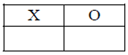
The Game will start with the empty matrix, like the following:

The Computer begins by placing an X in a location:

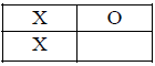
The player then clicks on one location, and in so doing changes the value of the button text from a null string to an O. The button must also be disabled so that a subsequent click cannot change it.
The Computer then selects a place to put another X (initially set so it will always win) and this matrix location receives the X and its button is disabled. (The original X should have been disabled at the beginning.)
The application will pop up a two button dialog box saying “I Have Won”. The two buttons on the dialog box should say “Play Again” and “Quit”, where “Quit” stops the program and “Play Again” clears the board and allows you to play again. You should also add a button on the Front Panel, “Restart” which will clear the board and restart.
In order to simplify the game, we will make two changes:
1. The computer starts first, and always moves in the upper left corner with an X.
2. The computer stops as soon as it wins.
To do this lab you will have to do multiple things:
1. Learn how to dynamically change the names on the OK buttons, and disable.
a. Setup: Do this by creating Property Nodes for each button (right click while in the Front Panel, under “Create”. On the Block Diagram you need to add another element to each property node (right-click, choose “Add Element”). Then set one element to “Disabled”, the other to `BoolText.text' by searching through the “Properties” menu on a right click. Change both elements to write.
b. Changing strings: You should now be able to attach a string to the “Booltext.text” and display it in the button when you run the program. To make a selection, build an array of strings, and select a single element of the array with an index. Set the array of strings to be “X”, “O”, and “ ” (an empty string). Test with a numeric control (make it U8!): when the program runs change the values of the numeric control to select different values of the text to be displayed on the button.
c. Disabling: Add a Boolean switch. In the dialog box, convert the Boolean value to a number using the “Boolean to (0:1)” function. Send the output of this to the Disable element of the button. If one passes a 0 to the Disable element, the button behaves normally. If one passes a 1, it is disabled. (FYI, if a 2 is passed to the button, the button is grayed out and disabled). By running the application you should be able to enable or disable the button at will, as well as change its caption.
2. Design a finite state machine on paper.
a. Work through the states of a FWM which compromise the Tic-Tac game. Start by assuming an unchecked space has a 0, a space with an X has a 1, and a space with an O has a 2. Each state could then have a label abcd, as below.
b. What is the initial state? Draw a circle for this one and label with
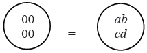
So this is state abcd = 0000. (The labels following the pattern of buttons.)
c. What are the first four possible states (primary states)? In a row below the initial state, draw a circle for each primary state and provide a label. For instance, if there is an X in upper left corner, the primary state would be labeled as

This is therefore state abcd = 1000. Draw an arrow from the initial state to each of the four different possible primary states.
d. Now draw a row of secondary states below the row of primary states. We will simplify by following only one of the primary states in this lab, otherwise the number of states grows tremendously. So for only state abcd = 1000 out of the first possible initial states, define the secondary states. For instance if the player chooses to move into bottom left, this would be a state abcd = 1020.

Each secondary state should be unique, but there may be arrows from two different primary states to
a single secondary state.
e. Now define the third level states and fourth level states. Note that the computer can win in every case, so the third level states are essentially predefined for two of the secondary states, but one of the secondary states has two different third state possibilities. There is only one fourth level state, where the computer prints out its victory message and waits.
3. Now that you have the state diagram, you have a certain number of unique states. Assign each of the above states a number. This is an arbitrary assignment and does not have to be in any order. The easiest way to do this is to name them abcd, i.e. state 1020, 2010, 1120, 0010, etc. In this case you have almost no work to do. Note that state 0000 would be interpreted by the Case Structure in LabVIEW as state 0. (One could use strings of the numbers to select as well actual numbers). The final victor state can be any number you have not already used; e.g. 9999.
4. Use a Case Structure imbedded within a While Loop to generate the finite element machine that jumps between the various states. In each state, assess what the input data is (the values of each of the 4 buttons in the matrix as well as the “Restart” switch) and select the next state to jump to. Pass this state back to the case statement using a tunnel in the While Loop. If you choose to number the states as 1020, 2010, etc, then as you add each case to the case statement, and change the case value to these numbers. State 0000 would be interpreted as state 0.
a. You will need to have a sort of numeric scratch pad where you can write some data and store it as well as read it back. The strategy here will be to use a local variable. First create four numeric controls. Each represents the states of each of the 4 matrix check boxes. Give each controll a representation of U8. You can hide the numeric controls from being visible on the Front Panel by right clicking on the numeric control from the front panel, and selecting “Hide Control” (located under submenu “Advanced”). Int the Block Diagram, make sure these numeric controls are outside of the Case Structure which controls the finite state machine sequence, but inside the overall While Loop. Use these variables to select the caption of the individual matrix element buttons (using the Array select, as in the part 1) as well as to disable the matrix element buttons (check to see if the variable is non-zero; if it is, disable the button).
b. Go to your initial state abcd = 0000 in the Block Diagram. Right click on the data object to select Create→Local Variable. Drop a local variable for each of the four numerical controls buttons into the abcd = 0000 state. Assign all of these value 0, except a, which will have value 2. You can use numeric constants to assign these values. Setup the jump to the next state abcd = 1000
c. Go to next state: abcd = 1000. Again, add local variables for bcd into this case. Assign b,c,d from the b, c, and matrix switch values. Setup a new state to jump to based on these switch values. (Hint: form an integer P= a +2b + 4c , then pass this to a new case statement embedded within this particular case statement. Select what the next state will be depending upon P=0, P=1, P=2 & P=4 ).
5. One state will pop up a dialog box. Be sure to wire the cancel output to stop the program.
6. One state, abcd = 1002, will have two possible computer moves to win. Use a random number generator to select which path will occur. The random number generator makes a number between 0.0 and 1.0. So compare the random number with 0.5, if it is less, the jump to one state, if it is more, jump to each other.
7. Be sure to initialize the state of the machine to 0 outside the main while loop. You probably will want to initialize each of the numeric matrix values as well here.
8. Try using the debugging features of LabVIEW as they will help you to discover problems. In particular, it can help you trace through the steps that your finite state machine is progressing through, and help you to diagnose when you are not jumping to the correct state.
Add to Cart
View detail
The Front Panel of the game will be built with four “O” buttons from the Boolean Controls Palette. Place the four controls close together to make a matrix. The computer begins by placing an X in some location of the matrix. One then uses the buttons to click on them and then select the square to place an O into. If one gets two in a row one wins (diagonal does not count).
The Game will start with the empty matrix, like the following:
The Computer begins by placing an X in a location:
The player then clicks on one location, and in so doing changes the value of the button text from a null string to an O. The button must also be disabled so that a subsequent click cannot change it.
The Computer then selects a place to put another X (initially set so it will always win) and this matrix location receives the X and its button is disabled. (The original X should have been disabled at the beginning.)
The application will pop up a two button dialog box saying “I Have Won”. The two buttons on the dialog box should say “Play Again” and “Quit”, where “Quit” stops the program and “Play Again” clears the board and allows you to play again. You should also add a button on the Front Panel, “Restart” which will clear the board and restart.
In order to simplify the game, we will make two changes:
1. The computer starts first, and always moves in the upper left corner with an X.
2. The computer stops as soon as it wins.
To do this lab you will have to do multiple things:
1. Learn how to dynamically change the names on the OK buttons, and disable.
a. Setup: Do this by creating Property Nodes for each button (right click while in the Front Panel, under “Create”. On the Block Diagram you need to add another element to each property node (right-click, choose “Add Element”). Then set one element to “Disabled”, the other to `BoolText.text' by searching through the “Properties” menu on a right click. Change both elements to write.
b. Changing strings: You should now be able to attach a string to the “Booltext.text” and display it in the button when you run the program. To make a selection, build an array of strings, and select a single element of the array with an index. Set the array of strings to be “X”, “O”, and “ ” (an empty string). Test with a numeric control (make it U8!): when the program runs change the values of the numeric control to select different values of the text to be displayed on the button.
c. Disabling: Add a Boolean switch. In the dialog box, convert the Boolean value to a number using the “Boolean to (0:1)” function. Send the output of this to the Disable element of the button. If one passes a 0 to the Disable element, the button behaves normally. If one passes a 1, it is disabled. (FYI, if a 2 is passed to the button, the button is grayed out and disabled). By running the application you should be able to enable or disable the button at will, as well as change its caption.
2. Design a finite state machine on paper.
a. Work through the states of a FWM which compromise the Tic-Tac game. Start by assuming an unchecked space has a 0, a space with an X has a 1, and a space with an O has a 2. Each state could then have a label abcd, as below.
b. What is the initial state? Draw a circle for this one and label with
So this is state abcd = 0000. (The labels following the pattern of buttons.)
c. What are the first four possible states (primary states)? In a row below the initial state, draw a circle for each primary state and provide a label. For instance, if there is an X in upper left corner, the primary state would be labeled as
This is therefore state abcd = 1000. Draw an arrow from the initial state to each of the four different possible primary states.
d. Now draw a row of secondary states below the row of primary states. We will simplify by following only one of the primary states in this lab, otherwise the number of states grows tremendously. So for only state abcd = 1000 out of the first possible initial states, define the secondary states. For instance if the player chooses to move into bottom left, this would be a state abcd = 1020.
Each secondary state should be unique, but there may be arrows from two different primary states to
a single secondary state.
e. Now define the third level states and fourth level states. Note that the computer can win in every case, so the third level states are essentially predefined for two of the secondary states, but one of the secondary states has two different third state possibilities. There is only one fourth level state, where the computer prints out its victory message and waits.
3. Now that you have the state diagram, you have a certain number of unique states. Assign each of the above states a number. This is an arbitrary assignment and does not have to be in any order. The easiest way to do this is to name them abcd, i.e. state 1020, 2010, 1120, 0010, etc. In this case you have almost no work to do. Note that state 0000 would be interpreted by the Case Structure in LabVIEW as state 0. (One could use strings of the numbers to select as well actual numbers). The final victor state can be any number you have not already used; e.g. 9999.
4. Use a Case Structure imbedded within a While Loop to generate the finite element machine that jumps between the various states. In each state, assess what the input data is (the values of each of the 4 buttons in the matrix as well as the “Restart” switch) and select the next state to jump to. Pass this state back to the case statement using a tunnel in the While Loop. If you choose to number the states as 1020, 2010, etc, then as you add each case to the case statement, and change the case value to these numbers. State 0000 would be interpreted as state 0.
a. You will need to have a sort of numeric scratch pad where you can write some data and store it as well as read it back. The strategy here will be to use a local variable. First create four numeric controls. Each represents the states of each of the 4 matrix check boxes. Give each controll a representation of U8. You can hide the numeric controls from being visible on the Front Panel by right clicking on the numeric control from the front panel, and selecting “Hide Control” (located under submenu “Advanced”). Int the Block Diagram, make sure these numeric controls are outside of the Case Structure which controls the finite state machine sequence, but inside the overall While Loop. Use these variables to select the caption of the individual matrix element buttons (using the Array select, as in the part 1) as well as to disable the matrix element buttons (check to see if the variable is non-zero; if it is, disable the button).
b. Go to your initial state abcd = 0000 in the Block Diagram. Right click on the data object to select Create→Local Variable. Drop a local variable for each of the four numerical controls buttons into the abcd = 0000 state. Assign all of these value 0, except a, which will have value 2. You can use numeric constants to assign these values. Setup the jump to the next state abcd = 1000
c. Go to next state: abcd = 1000. Again, add local variables for bcd into this case. Assign b,c,d from the b, c, and matrix switch values. Setup a new state to jump to based on these switch values. (Hint: form an integer P= a +2b + 4c , then pass this to a new case statement embedded within this particular case statement. Select what the next state will be depending upon P=0, P=1, P=2 & P=4 ).
5. One state will pop up a dialog box. Be sure to wire the cancel output to stop the program.
6. One state, abcd = 1002, will have two possible computer moves to win. Use a random number generator to select which path will occur. The random number generator makes a number between 0.0 and 1.0. So compare the random number with 0.5, if it is less, the jump to one state, if it is more, jump to each other.
7. Be sure to initialize the state of the machine to 0 outside the main while loop. You probably will want to initialize each of the numeric matrix values as well here.
8. Try using the debugging features of LabVIEW as they will help you to discover problems. In particular, it can help you trace through the steps that your finite state machine is progressing through, and help you to diagnose when you are not jumping to the correct state.
Lab .2(b): Additional LabVIEW Exercises
In this lab you will continue to explore the LabVIEW. You must complete 8 of the following 15 exercises.
1. Build a VI that compares two numbers and turns on an LED if the first number is greater than or equal to the second number. Tip: Use the Greater Or Equal? function located on the Functions»Comparison palette.
Save the VI as Compare.vi
2. Build a VI that generates a random number between 0.0 and 10.0 and divides the random number by a number specified on the front panel. If the number input is 0, the VI should turn on a front panel LED to indicate a divide by zero error.
Save the VI as Divide.vi
3. Using only a While Loop, build a combination For Loop and While Loop that stops either when it reaches a number of iterations specified with a front panel control, or when you click a stop button.
Save the VI as Combo While-For Loop.vi
4. Build a VI that continuously measures the temperature once per second and displays the temperature on a scope chart. If the temperature goes above or below limits specified with front panel controls, the VI turns on a front panel LED. The chart plots the temperature and the upper and lower temperature limits. You should be able to set the limit from the following front panel.
Save the VI as Temperature Limit.vi
5. Modify the VI you created in Exercise 4 to display the maximum and minimum values of the temperature trace. Tip: Use shift registers and two Max & Min functions located on the Functions»Comparison palette.
Save the VI as Temp Limit (max-min).vi
6. Build a VI that reverses the order of an array containing 100 random numbers. For example, array[0] becomes array[99], array[1] becomes array[98], and so on. Tip: Use the Reverse 1D Array function located on the Functions»Array palette to reverse the array order.
Save the VI as Reverse Random Array.vi
7. Build a VI that first accumulates an array of temperature values using the Thermometer VI, which you have already built. Set the array size with a control on the front panel. Initialize an array using the Initialize Array function of the same size where all the values are equal to 10. Add the two arrays, calculate the size of the final array, and extract the middle value from the final array. Display the Temperature Array, Initialized Array, Final Array, and Mid Value.
Save the VI as Find Mid Value.vi
8. Build a VI that generates a 2D array of three rows by 10 columns containing random numbers. After generating the array, index each row and plot each row on its own graph. The front panel should contain three graphs.
Save the VI as Extract 2D Array.vi
9. Build a VI that simulates the roll of a die with possible values 1–6 and records the number of times that the die rolls each value. The input is the number of times to roll the die and the outputs include the number of times the die falls on each possible value. Use only one shift register.
Save the VI as Die Roller.vi
10. Build a VI that generates a 1D array and then multiplies pairs of elements together, starting with elements 0 and 1, and returns the resulting array. For example, the input array with values 1 23 10 5 7 11 results in the output array 23 50 77. Tip: Use the Decimate 1D Array function located on the Functions»Array palette.
Save the VI as Array Pair Multiplier.vi
11. Build a VI that uses the Formula Node to calculate the following equations:

Add to Cart
View detail
1. Build a VI that compares two numbers and turns on an LED if the first number is greater than or equal to the second number. Tip: Use the Greater Or Equal? function located on the Functions»Comparison palette.
Save the VI as Compare.vi
2. Build a VI that generates a random number between 0.0 and 10.0 and divides the random number by a number specified on the front panel. If the number input is 0, the VI should turn on a front panel LED to indicate a divide by zero error.
Save the VI as Divide.vi
3. Using only a While Loop, build a combination For Loop and While Loop that stops either when it reaches a number of iterations specified with a front panel control, or when you click a stop button.
Save the VI as Combo While-For Loop.vi
4. Build a VI that continuously measures the temperature once per second and displays the temperature on a scope chart. If the temperature goes above or below limits specified with front panel controls, the VI turns on a front panel LED. The chart plots the temperature and the upper and lower temperature limits. You should be able to set the limit from the following front panel.
Save the VI as Temperature Limit.vi
5. Modify the VI you created in Exercise 4 to display the maximum and minimum values of the temperature trace. Tip: Use shift registers and two Max & Min functions located on the Functions»Comparison palette.
Save the VI as Temp Limit (max-min).vi
6. Build a VI that reverses the order of an array containing 100 random numbers. For example, array[0] becomes array[99], array[1] becomes array[98], and so on. Tip: Use the Reverse 1D Array function located on the Functions»Array palette to reverse the array order.
Save the VI as Reverse Random Array.vi
7. Build a VI that first accumulates an array of temperature values using the Thermometer VI, which you have already built. Set the array size with a control on the front panel. Initialize an array using the Initialize Array function of the same size where all the values are equal to 10. Add the two arrays, calculate the size of the final array, and extract the middle value from the final array. Display the Temperature Array, Initialized Array, Final Array, and Mid Value.
Save the VI as Find Mid Value.vi
8. Build a VI that generates a 2D array of three rows by 10 columns containing random numbers. After generating the array, index each row and plot each row on its own graph. The front panel should contain three graphs.
Save the VI as Extract 2D Array.vi
9. Build a VI that simulates the roll of a die with possible values 1–6 and records the number of times that the die rolls each value. The input is the number of times to roll the die and the outputs include the number of times the die falls on each possible value. Use only one shift register.
Save the VI as Die Roller.vi
10. Build a VI that generates a 1D array and then multiplies pairs of elements together, starting with elements 0 and 1, and returns the resulting array. For example, the input array with values 1 23 10 5 7 11 results in the output array 23 50 77. Tip: Use the Decimate 1D Array function located on the Functions»Array palette.
Save the VI as Array Pair Multiplier.vi
11. Build a VI that uses the Formula Node to calculate the following equations:

Use only one Formula Node for both equations and use a semicolon (;) after each equation in the node.
Save the VI as Equations.vi
12. Build a VI that functions like a calculator. On the front panel, use digital controls to input two numbers and a digital indicator to display the result of the operation (Add, Subtract, Divide, or Multiply) that the VI performs on the two numbers. Use a slide control to specify the operation to perform.
Save the VI as Calculator.vi
13.Build a VI that has two inputs, Threshold and Input Array, and one output, Output Array. contains values from that are greater than.
Save the VI as Array Over Threshold.vi
Create another VI that generates an array of random numbers between 0 and 1 and uses the Array Over Threshold VI to output an array with the values greater than 0.5.
Save the VI as Using Array Over Threshold.vi
14. Build a VI that generates a 2D array of 3 rows 100 columns of random numbers and writes the data transposed to a spreadsheet file. Add a header to each column. Use the high-level File I/O VIs located on the Functions»File I/O palette. Tip: Use the Write Characters To File VI to write the header and the Write To Spreadsheet File VI to write the numeric data to the same file.
Save the VI as More Spreadsheets.vi
15. Build a VI that converts tab-delimited spreadsheet strings to comma-delimited spreadsheet strings, that is, spreadsheet strings with columns separated by commas and rows separated by end of line characters. Display both the tab-delimited and comma-delimited spreadsheet strings on the front panel. Tip: Use the Search and Replace String function.
Save the VI as Spreadsheet Converter.vi
Lab .1 (a) - Beginning LabVIEW Programming
1.Create an application which reads the current time from the computer, and pops up a simple dialog box with the time information.
a.Create new LabVIEW application. Go to the Block Diagram, and show the Functions Palette.
b.On the Functions Palette put a copy of the function “Get Date/Time in Seconds” (under “Time and Dialog”) onto your diagram. Also get a copy of the function “Format Date/Time String” from the same palette. Connect them up to create a text formatted string with the current date and time.
c.Under “String” get the string concatenation function. Concatenate the previous text string, containing the current date and time, to the end of a new text string constant containing the words “The current date and time is: ”.
d.Create a Single Button Dialog Box (a function under “Time and Dialog”). Use the text string from part (1c) as the text for the Dialog Box. Use another text string constant to make a name, “Thanks”, for the title of the dialog box button.
e.When you run the program, it should pop-up a single dialog box which says “The Current date and time is: XXXX" where XXXX is the current date and time. Clicking on the “Thanks” button will close the dialog box. Demonstrate the program to the TA.
2. Create an application which reads a text string from the Control Panel, and sends the text string to a text string display as well as to a dialog box.
Add to Cart
View detail
a.Create new LabVIEW application. Go to the Block Diagram, and show the Functions Palette.
b.On the Functions Palette put a copy of the function “Get Date/Time in Seconds” (under “Time and Dialog”) onto your diagram. Also get a copy of the function “Format Date/Time String” from the same palette. Connect them up to create a text formatted string with the current date and time.
c.Under “String” get the string concatenation function. Concatenate the previous text string, containing the current date and time, to the end of a new text string constant containing the words “The current date and time is: ”.
d.Create a Single Button Dialog Box (a function under “Time and Dialog”). Use the text string from part (1c) as the text for the Dialog Box. Use another text string constant to make a name, “Thanks”, for the title of the dialog box button.
e.When you run the program, it should pop-up a single dialog box which says “The Current date and time is: XXXX" where XXXX is the current date and time. Clicking on the “Thanks” button will close the dialog box. Demonstrate the program to the TA.
2. Create an application which reads a text string from the Control Panel, and sends the text string to a text string display as well as to a dialog box.
a. Create a new LabVIEW application. Go to the Front Panel, and add a String Control and a String Indicator to the panel. Rename the String Control as “Input”. Rename the String Indicator as “Output”.
b. On the Block Diagram, wire the String Control to the String Indicator. Go back to the Front Pane, type some text into each input area (different text data in each). Run the program. Which input text changes? Which text stays the same?
c. On the Front Panel add a single LED Indicator (under “Boolean”). On the Block Diagram add a “Two-Button Dialog”. Connect the return value from the dialog box (“T?”) to the LED Indicator. Pass the string from the “Input” String Control to the name of the dialog box, but do it so that all characters are capital letters. Do this by sending the string from the string control through the “To Upper Case” function in the String Palette. The output from this function is then sent to the dialog box name input. Save the application at this point, you may lose the LabVIEW application if you click on the wrong “run” button in part (2d).
d. Test by entering some lower case data into the “Input” area on the Front Panel, then running the program using the “Run Once” button. DO NOT use the continuous run mode of LabVIEW. The dialog box should appear with the text string in upper case. If you click on “OK” the LED should turn on. If you click on “Cancel” the LED should turn off.
e. Be sure you have saved the application. After having saved the application, try hitting the “Continuous Run” button. What happens? Is there any way to stop the program?
f. Hit Ctrl-Alt-Delete to bring up the Windows Task Manager, select LabVIEW, and then select End Task. This is the only way to stop the process. Restart LabVIEW and reload your saved program. Do not run it.
g. We will now fix this lockup problem. In general, you should always test your software to make sure somebody cannot lock up the system by pressing the wrong run button. To fix the problem, you need to stop the program when the person clicks on one of the dialog box buttons. Go to the Block Diagram. In the Functions Palette, look in “Application Control” for a stop sign. Put the stop sign on the Block Diagram and connect the input to the Boolean output from the dialog box. The stop sign will stop the program if it receives a true; the program keeps running if the stop sign receives a false. Save the program, then try to
run in both run-once mode and in continuous mode. The program should exit nicely when you click on the correct dialog box button (OK).
run in both run-once mode and in continuous mode. The program should exit nicely when you click on the correct dialog box button (OK).
3. Create a Boolean-to-decimal converter, and identify the difference between I8 and U8 integers.
a. Create a new LabVIEW application. Place eight vertical toggle switches in a roughly straight horizontal line on the Front Panel. Select all eight switches with a selection box. Use “Distribute Objects” and “Horizontal Center” to distribute the switches evenly in the line, then use the “Align Objects” to align all the switches on their vertical centers. The result should have all the switches neatly aligned and evenly spaced.
b. Rename the switch titles, from left to right , as “128”, “64”, “32”, “16”, “8”, “4”, “2”, and “1”.
c. Go to the Block Diagram. Align the eight Boolean outputs as you did for the switches in part (3a).
d. We will take these individual bits from the switches and concatenate them together to form a single byte. Each switch will then control the value of a different bit of the byte. To form the byte, use the “Build Array” function from the Functions Palette in the Block Diagram. Drop one of these objects into your Diagram. Add seven more inputs by placing the arrow tool into the left hand side of this function, then right-clicking with your mouse to select the “Add Input” function. Add seven more inputs so the total number of inputs is eight.
e. Wire the switch outputs, in sequential order, to the inputs of the build array. Note that the bottom-most input of the array will be the leftmost bit, the one corresponding to the 128's bit; the topmost input will be the rightmost bit, corresponding to the 1's bit.
f. Convert this array into a number using the “Boolean array to number” function under "Numeric", submenu "Conversion"
g. On the Front Panel, add a Digital Indicator (under "Numeric").
h. Go to the Block Diagram. You now need to set the type of data to be displayed by the numeric control. Point to the Numeric Indicator (in yellow, says “DBL”), right click and select submenu “Representation”. This is currently set to “DBL” meaning double precision floating point. Change this to “U8” meaning unsigned byte.
i. Run the program from the Front Panel, and click the switches to different states. Verify that the numeric output is the proper sum of the individual bit values. In particular, see what happens when you click the 128 switch on and off. What is the biggest number you can get? What is the smallest?
j. Now go to the Block Diagram, and change the data type from “U8” to “I8” meaning signed byte.
k. Run the program from the Front Panel, and click the switches to different states. Verify that the numeric output is the proper sum of the individual bit values. In particular, see what happens when you click the 128 switch on and off. What is the biggest number you can get? What is the smallest?
l. In (3h), if one changed U8 to U16 or U32, would it make any difference? What would the minimum/maximum that could be displayed be as the eight switches were toggled?
m. In (3k), if one changed U8 to I16 or I32, would it make any difference? What would the minimum/maximum that could be displayed be as the eight switches were toggled?
Thursday, August 16, 2012
Lab .4 (a) How to Use an Oscilloscope in LabVIEW
LabVIEW, developed by National Instruments, is a graphical programming environment used by engineers to create and test complex measurement, test and control systems. LabVIEW can use thousands of hardware devices to provide data visualization. If you want to use your oscilloscope to measure the voltage and frequency of an electric signal and have the data displayed in LabVIEW, you must first properly connect to it using the National Instruments Measurement and Automation Explorer (MAX) tool. Once your oscilloscope is recognized, you can add it to your LabVIEW project and receive and use data in real time.
Instructions
1. Turn on the oscilloscope, and connect it to your computer.
Add to Cart
View detail
Instructions
1. Turn on the oscilloscope, and connect it to your computer.
2. Start the Measurement and Automation Explorer tool.
3. Right-click on "Devices and Interfaces," and select the "Create New" option.
3. Right-click on "Devices and Interfaces," and select the "Create New" option.
4. Click on the "VISA TCP/IP Resource" item in the list, and click "Next."
5. Select the "Auto-detect of LAN instrument" option, and click "Next." MAX searches and locates your oscilloscope. Select it, and click "Next."
6. Type a VISA alias that will act as the name of your instrument, and click "Finish." The oscilloscope appears under the VISA TCP/IP Resource section and can be accessed from LabVIEW.
7. Start LabVIEW, and open or create a project.
8. Open the Controls toolbox in LabVIEW, and click on the "I/O" button to display the I/O devices.
9. Click on the "VISA resource" button to display a list of all VISA devices. Note that your oscilloscope is listed under the VISA alias you selected earlier.
10. Drag the oscilloscope VISA resource onto your LabVIEW project to insert it. The device should communicate with LabVIEW properly as long as the connection is active and the device is turned on.
11. Use the oscilloscope to measure the voltage and frequency of your electric signal, and the data will be displayed in LabVIEW.
Sponsored Links
Sponsored Links
Lab .4 (c) How to Measure Signal Change in LabVIEW
LabVIEW is primarily a data acquisition software that allows collection, analysis, storage and retrieval of massive amounts of data. LabVIEW supports function blocks that are specifically developed to work with data acquisition cards that are developed by National Instruments. Measurement and Automation Explorer (MAX) is a software distributed along with LabVIEW that allows users to configure the data acquisition hardware to easily read signals in LabVIEW programs.
Instructions
Setting up a Global Virtual Channel to Read Signal in MAX Software
Add to Cart
View detail
Instructions
Setting up a Global Virtual Channel to Read Signal in MAX Software
1. Launch the MAX software. In the "Configuration" pane, click on "Devices and Interfaces," "NI-DAQmx Devices" to display a list of all the data acquisition cards that are installed on the computer. For example, if PCI-6122 is installed, the list will show "NI PCI-6122: Dev1" in the list. The "Dev1" is a reference that is used in the LabVIEW VI program to access the input channel of the card to read signal values.
2. Click on "Data Neighbourhood" in the configuration pane to display "NI-DAQmx Global Virtual Channels." Right-click on "NI-DAQmx Global Virtual Channels" and click on "Create New NI-DAQmx channel."
3. Click on "Acquire Signal/Analog Input/Voltage" in the "Create New NI-DAQmx Global Virtual Channel" window to list all the physical channels on "Dev1" board that can be accessed to read input signals. Click on "port1/ai0" to choose "ai0" as the input channel. Click "Next" and enter the name "myInput." Click "Finish." MAX software will display a window showing "Dev1/port0/line0" as the configured global virtual channel for an analog input on board PCI-6122. The global virtual channel is called "myInput" and will be used in LabVIEW to read signals.
Using a Global Virtual Channel in a LabVIEW Program
4. Launch LabVIEW and click on "New VI" in the resulting splash screen to create a new LabVIEW VI program. Every LabVIEW VI has two windows: the front panel window and the diagram window.
5. Drag and drop the "DAQmx Global Virtual Channel" control and "Numeric" indicator from the "Controls" pallet in the front panel window. All components dropped on the front panel will also show up in diagram window of the VI. In the diagram window, drag and drop the "DAQmx read" component from the "Functions" pallet.
6. Connect the output "DAQmx Global Virtual Channel" control to the "Virtual Channel In" input of the "DAQmx Read" component. Connect the output of the "DAQmx Read" component to the input of the "Numeric" component.
7. Choose "myInput" on the "DAQmx Global Virtual Channel" control in the front panel window. Click "Continuous Run VI" button on the "menu" bar on the top of the front panel. Any change to the signal connected to the data acquisition card on channel "ai0" will be continuously displayed in the "Numeric" indicator.
Lab .4 (b) How to Measure Sound Signals Using LabVIEW
The LabVIEW software platform allows engineers to create a wide variety of virtual instruments, or VI, that allow the analysis, testing and design of different machines. Measuring sound is ideally done with the LabVIEW add on, Sound and Vibration Toolkit, which provides several VI for measuring sound signals. Depending on what kind of input you want to measure and the output that provides useful data, there are unlimited configurations within LabVIEW. However; the basic setup for each type of measurement you perform is the same.
Instructions
Sound Signals Measurement Setup
1. Determine the sound signals you want to measure and pick a virtual instrument within LabVIEW to produce the sound, or a real-world sound producer such as a microphone. Attach your sound device to the computer, if applicable.
Add to Cart
View detail
Instructions
Sound Signals Measurement Setup
1. Determine the sound signals you want to measure and pick a virtual instrument within LabVIEW to produce the sound, or a real-world sound producer such as a microphone. Attach your sound device to the computer, if applicable.
2. Launch LabVIEW, then click "Blank VI." Build your VI in the diagram by connecting three types of elements from left to right: an input device, which may be a real audio instrument or a virtual instrument in LabVIEW, a LabVIEW measurement device, and an output device in LabVIEW. There are unlimited combinations. Pick the devices that measure sound based on your requirements. For example; use the "Tone Measurement" device and "Fundamental Tone" output device to measure frequency and amplitude of an input signal.
3. Right-click on the output device in your block diagram, then click "Create." Pick the name of the indicator from the Sound and Vibration palette, such as "Waveform," to display a graphical representation of the sound measurement on the front panel.
Configuring LabVIEW to Measure Hardware Input
3. Right-click on the output device in your block diagram, then click "Create." Pick the name of the indicator from the Sound and Vibration palette, such as "Waveform," to display a graphical representation of the sound measurement on the front panel.
Configuring LabVIEW to Measure Hardware Input
4. Launch Measurement & Automation Explorer (MAX) by clicking on the application in the "LabView" folder in the "Programs" list.
5. Click "NI-DAQmx Devices, then click "Create New DAQmx Device, and click "NI-DAQmx Simulated Device."
6. Click on the arrow next to the "USB DAQ" menu, then click "USB-9233." This prepares LabVIEW to accept an analog input through an audio optimized USB driver.
7. Right-click on "Data Neighborhood" in the MAX configuration list and click "Create New."
8. Click on "NI-DAQmx Task" and click "Next."
9. Click on the "Analog Input" drop down menu, then click "Sound Pressure." In the list that appears, click "ai0" under "USB-9233" and click "Next."
10. Type the name of your analog signal in the text box, then click "Finish." LabVIEW is ready to accept your sound device as an input signal.
Lab .5(a) How to Import CSV to LabVIEW
Comma Separated Values, or CSV, is a format in which strings are saved in a text file. In this format, values are saved in string format in multiple rows. Each row consists of multiple values separated by commas as delimiters. These commas can be used as means to separate values from each row. Reading CSV files into LabVIEW is a common task that enables you to read data or values stored in CSV files in an easy and convenient way.
Instructions
1. A CSV file consists of comma separated data stored in multiple lines. The following lines are an example of the contents of a CSV file;
This,Is,Line,One
This,Is,Line,Two
This,Is,Line,Three
As an example, assume that the lines are saved in a CSV file called as "myData.csv."
Add to Cart
View detail
Instructions
1. A CSV file consists of comma separated data stored in multiple lines. The following lines are an example of the contents of a CSV file;
This,Is,Line,One
This,Is,Line,Two
This,Is,Line,Three
As an example, assume that the lines are saved in a CSV file called as "myData.csv."
2. Launch LabVIEW 8 software, create a new VI by clicking on "New VI" in the splash window. Save it as "importCSV.vi." In the diagram window for the "importCSV.vi," drag and drop the following components from the Funtionals Palette; "Read From Text File," "Spreadsheet String to Array" and "Line Feed" constant from the strings palette.
3. The "Read From Text File" block accepts as an input the file path to the CSV file. Right click on the block and from the list that pops up, click on "Create Constant" for the file path input. Type the complete path to the CSV file in the constant. For example, if the "myData.csv" file is located on the "C" drive, type "C:\myData.csv" in the "File Path" constant.
The output of the "Read From Text File" block is a text string commonly known as a spreadsheet string. This spreadsheet string consists of all the contents of the CSV file.
4. Connect the output string from the previous step to the input of "Spreadsheet String to Array" block. The output of "Spreadsheet String to Array" block is an array of strings. Use the "Line Feed" constant as a delimiter to separate the rows into a single dimension array of strings by connecting it to the "Delimiter" input of the "Spreadsheet String to Array" block. Each row is separated and populated into the array as an individual string element of the array.
5. Create a For Loop in the diagram window of the LabVIEW program. Connect the array of individual rows to the For Loop. Right click at the point where the array is connected to the For Loop and select "Enable Indexing." This ensures that for each iteration of the For Loop only one element from the array is accepted as input. It will also ensure that the number of For Loop iterations will be equal to the size of the array.
Inside the For Loop use another "Spreadsheet String to Array" block. This time use a comma as a delimiter. In every For Loop iteration a different row will be parsed into an array of string elements. The values from the CSV file import into LabVIEW as a single chunk of data, separated into individual rows and then parsed into separate values.
Inside the For Loop use another "Spreadsheet String to Array" block. This time use a comma as a delimiter. In every For Loop iteration a different row will be parsed into an array of string elements. The values from the CSV file import into LabVIEW as a single chunk of data, separated into individual rows and then parsed into separate values.
Lab .5(b) How to Use Excel With LabVIEW
Microsoft Excel is a popular spreadsheet software used by professionals in every field from finance to biology. The program is used to analyze data, among other tasks. National Instruments' LabVIEW is one of the leading tool kits for data collection, sensor management and other laboratory experiment automation. By using Excel and LabVIEW in concert, you can improve your overall work flow and make both recording and analysis a breeze.
Instructions
1. Create a new virtual instrument (VI) in LabVIEW, or open an existing one.
Add to Cart
View detail
Instructions
1. Create a new virtual instrument (VI) in LabVIEW, or open an existing one.
2. Add your sensors to the VI. You can also add any other elements you want; they will run simultaneously with the spreadsheet export.
If you don't know what sensors you'll be using yet, you can test out your Excel integration by using a clock as the "sensor". To do this, go to the Functions window, expand the Utilities palette, and drag the Clock element into the main LabVIEW window.
3. Go to the Functions window, and expand the File I/O palette. Drag the "Write To Spreadsheet File" element into the main LabVIEW window near your sensor(s).
4. Go to the Tools menu and click "Connect Wire," which is the left-center button in the main block of 9 tools and has an icon that looks like a spool of wire. This will turn your mouse cursor into a wiring tool. Click on the sensor whose output you want to put in your spreadsheet, and drag the wiring tool onto the "Write To Spreadsheet File" element; release your mouse button. This will connect the output of the sensor to the input of the "Write To Spreadsheet File" element.
5. Drag a Path element out of the File I/O palette in the Functions window, if you would like to set a fixed location for the spreadsheet file to be saved. Connect it using the wiring tool (see Step 4). Double-click your Path element and enter the path where you would like to save the file. If you omit this step, LabVIEW will ask you where to save the spreadsheet each time you run the VI.
6. Run your VI. It will save your data to the Excel file you chose in Step 5.
7. Open the spreadsheet file in Excel. You can now use all the normal Excel data analysis tools on your sensor readouts.
Lab .5(c) How to Read From a Spreadsheet in LabVIEW
LabVIEW is a graphical programming application distributed by National Instruments. The program is used for designing components and systems in the science and engineering fields. LabVIEW offers compatible versions for all operating systems.LabVIEW provides the user with the ability to perform data visualization and analysis using datasets. To read data from a spreadsheet in LabVIEW, use the "Read From Spreadsheet File" VI. Convert the spreadsheet to Comma Separated Value (CSV) format and import the data into LabVIEW.
Instructions
1. Open the spreadsheet in its native application. For example, if the spreadsheet is a Microsoft Excel file, open the dataset in Microsoft Excel.
Add to Cart
View detail
Instructions
1. Open the spreadsheet in its native application. For example, if the spreadsheet is a Microsoft Excel file, open the dataset in Microsoft Excel.
2. Click the "File" option from the top navigation bar, or click the Microsoft Office button in Excel 2007, then click "Save As."
3. Click "Other Formats," then click the "Save as Type" drop-down box. Select the "CSV Comma Delimited (.csv)" file type, and click "Save." The dataset saves in the CSV format.
3. Click "Other Formats," then click the "Save as Type" drop-down box. Select the "CSV Comma Delimited (.csv)" file type, and click "Save." The dataset saves in the CSV format.
4. Click the "Functions" option in LabVIEW to open the "Functions" interface.
5. Click the "File I/O" icon, then click "Read From Spreadsheet File.vi" from the File I/O options.
6. Right-click on the "Delimiter Input" option located at the bottom of the window.
7. Click "Create," and click "Constant."
8. Type a comma (",") in the "String Constant" field. A file navigation window opens.
9. Navigate to the spreadsheet file saved in CSV format. Click on the file, and click "Open." The dataset loads into LabVIEW.
Lab .3(b) How to Make a Circle in LabVIEW
The graphical user interface that LabVIEW provides for the development of software applications allows users to develop applications faster. LabVIEW provides a set of functions that can be used to draw various shapes. These shapes are drawn as pictures on the front panel window of a LabVIEW program. A built in function block called "Draw Circle by Radius.VI" can be used to draw a circle in LabVIEW.
Instructions
1. Double-click on the LabVIEW shortcut on your desktop to launch the program. Click on "New VI" to launch a new LabVIEW program with two windows: the diagram window to develop the graphical code and the front panel window to develop the user interface. Save the program as "DrawCircle.VI."
Add to Cart
View detail
Instructions
1. Double-click on the LabVIEW shortcut on your desktop to launch the program. Click on "New VI" to launch a new LabVIEW program with two windows: the diagram window to develop the graphical code and the front panel window to develop the user interface. Save the program as "DrawCircle.VI."
2. Click on "View," "Functions Palette" on the "Menu" of the diagram window to open the functions palette. Drag and drop the "Draw Circle by Radius.VI" from the functions palette into the diagram window. This function block has an output called "New Picture" and two inputs called "Radius" and "Pixel Center."
3. Right-click on the "New Picture" output and click on "Create Indicator." A picture frame will automatically appear on the front panel window. Right click on each of the inputs and click on "Create Indicator" to create user input controls on the front panel window for entering the value of the radius and the location of the center of the circle.
3. Right-click on the "New Picture" output and click on "Create Indicator." A picture frame will automatically appear on the front panel window. Right click on each of the inputs and click on "Create Indicator" to create user input controls on the front panel window for entering the value of the radius and the location of the center of the circle.
4. Enter the value "20" in the input control called "Radius." The "Pixel Center" input has two sections: horizontal position and vertical position. Enter the value "20" in both sections.
5. Click on the "Run" button on the "Menu" bar of the front panel window to execute the program. A circle of radius 20 will be drawn in the picture frame. Change the value of the vertical and horizontal position to change the position of the circle in the picture frame.
Lab .3(b)How to Import a LabView Screen From CCI
National Instruments' LabVIEW graphical programming language fulfills many of the requirements for performing various laboratory experiments. The software's versatility is its most important quality. This is evident not only in the development of executable routines, which are called virtual instruments, but also in the ability to import and incorporate data files from peripheral hardware into these routines. Some file types are trickier to access than others. For example, files with a .cci extension are encoded using a communications protocol designed for use in fax machines. Importing a graph or screen from a .cci file and making it visible on the LabVIEW front panel might not be immediately intuitive, but LabVIEW's versatility can make this file usable, with the aid of the NI-IMAQ Vision software module.
Instructions
1. Start LabVIEW. On the top menu, left-click on the "File" tab to access the file menu. Select the "Create new .vi" option to create a blank virtual instrument. This opens two screens. The gray screen, or Front Panel, allows users to interface with an active program through buttons, switches, controls and indicators. The white screen, or Wiring Diagram, allows programmers to place and position icons, which contain previously established coded routines.
Add to Cart
View detail
Instructions
1. Start LabVIEW. On the top menu, left-click on the "File" tab to access the file menu. Select the "Create new .vi" option to create a blank virtual instrument. This opens two screens. The gray screen, or Front Panel, allows users to interface with an active program through buttons, switches, controls and indicators. The white screen, or Wiring Diagram, allows programmers to place and position icons, which contain previously established coded routines.
2. Position the cursor on any empty portion of the Wiring Diagram screen. Right click to access LabVIEW's toolbox; this is where you access the icon library. Select the "For Loop" and place this on the wiring diagram. Locate the green box near the lower right-hand corner inside the loop. This box contains the loop's properties. Right click on this box. Select the "Create Control" option. This places a Control marker on the Wiring Diagram and an "Off Button" on the Front Panel. When the program is running, the user can use this button to end the program.
3. Position the cursor on the Wiring Diagram screen outside the For Loop. Right click to access the LabVIEW toolbox. Select the "IMAQ initialization routine" icon to place it on the Wiring Diagram. Right click on the "IMAQ initialization" icon to access its properties. Set the constant to read information from a file directly to the clipboard.
3. Position the cursor on the Wiring Diagram screen outside the For Loop. Right click to access the LabVIEW toolbox. Select the "IMAQ initialization routine" icon to place it on the Wiring Diagram. Right click on the "IMAQ initialization" icon to access its properties. Set the constant to read information from a file directly to the clipboard.
4. Position the cursor inside the For Loop. Right click to access the LabVIEW toolbox. Select the "Read From Clipboard" and the "Write Waveform Graph" routines to place them on the Wiring Diagram. Right click on the "Write Waveform Graph" routine to access its properties and add a graph indicator to the output. This will add an icon to the Wiring Diagram and an image window to the Front Panel.
5. Left click on the "IMAQ initialization" routine to connect it to the "For Loop." This connection, known as a wire, determines the order of operations. Connect the "For Loop" tunnel to the "Read From Clipboard" icon input. Connect the "Read from Clipboard" output to the "Write Waveform Graph." The program is now ready to run from the front panel.
Lab .1(b) How to Measure Time on LabView
LabView is a software development platform that allows users to develop programs using a graphical language. LabView software applications are generally used for instrument control, machine automation and data acquisition. Many of these tasks require actions to be performed by the software at regular time intervals. For example, a data acquisition software may have to collect and save data points every two seconds. In such cases, the programmer has to write code to measure time using function blocks available in LabView.
Instructions
Add to Cart
View detail
Instructions
- Launch the LabView software by double-clicking on the LabView shortcut icon on your computer desktop. Create a new LabView program by clicking on "New VI" on the LabView splash screen, and save it as "measureTime.VI." Every LabView program has two windows: the front panel window and the diagram window.
- Open the "Functions" palette by clicking on "View" followed by "Functions palette" in the "Menu" bar of the diagram window. Drag and drop a "Time Elapsed" component from the "Functions" palette into the diagram window.
- Drag and drop a "While Loop" from the "Functions" palette around the "Time Elapsed" component. A stop button is automatically created for the while loop and is displayed on the front panel window. The "Time Elapsed" component has two outputs: the "Elapsed Time (s)" output and the "Present Time (s)" output.
- Right-click on the "Elapsed Time (s)" output and click on "Create Indicator." A numeric indicator for the elapsed time will be automatically displayed on the front panel window. Similarly, right-click on the "Present Time (s)" output. Click on "Create Indicator" to create a numeric indicator for displaying the present time on the front panel window.
- Run the LabView program by clicking on the "Run" button on the "Menu" bar of the front panel window. The "Elapsed Time" component will measure the time since the program started execution and display on the "Elapsed Time" numeric display on the front panel. The "Present Time" numeric display will show the current time.
Subscribe to:
Posts (Atom)


